Analog building blocks
Digital circuits use transistors as switches. Analog circuits use them as amplifiers: a small change at the gate makes a proportional change of drain current. Sensors, radios, audio, power management and every data converter are analog at heart. This chapter introduces the ideas behind every analog circuit, using the numbers of the generic 180 nm technology.
Bias first, then signal
An analog circuit is analysed in two steps:
- Bias (the DC operating point): fixed voltages and currents that put every transistor in saturation, where it behaves as a current source controlled by VGS (see the MOSFET).
- Small signal: small variations around that point. If they are small enough, the circuit is linear and simple formulas predict its gain.
In SPICE, step 1 is the operating point analysis and step 2 is the AC analysis, which linearises every device around its operating point.
Transconductance gm and output resistance ro
Two small-signal numbers describe a transistor in saturation:
-
Transconductance gm: how much the drain current changes per volt of gate voltage. From the square law:
g_m = ∂I_D/∂V_GS = 2·I_D / V_ov = √(2·k'·(W/L)·I_D)More current, or a smaller overdrive, gives more gm per microamp.
-
Output resistance ro: the flat curves of the saturation region are not perfectly flat. Their slope is the output conductance gds = 1/ro ≈ λ·ID. Longer transistors have a smaller λ and a higher ro.
After an operating-point simulation, IC Studio lists gm and gds for every transistor
on the Operating Point tab. Reading them is half of analog design.
The common-source amplifier
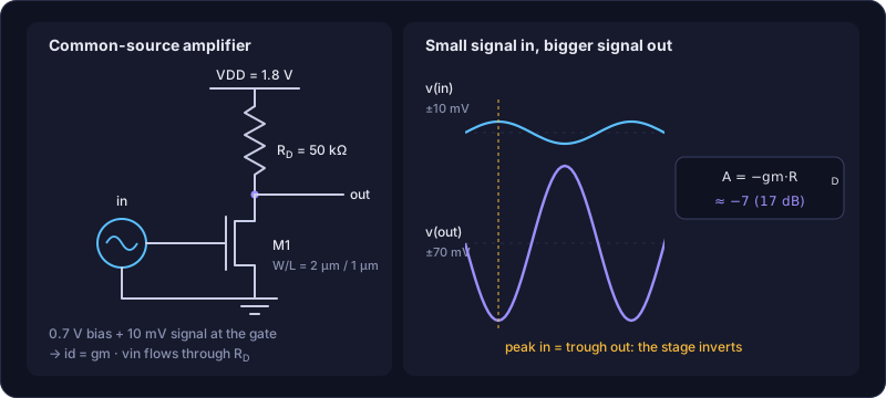
The basic amplifier: an NMOS with its source at ground, the input on its gate, and a load resistor RD from the drain to VDD.
- A small increase vin of the gate voltage increases the drain current by gm·vin.
- That extra current flows through RD and lowers the drain voltage by gm·vin·RD.
So the voltage gain is
A_v = v_out / v_in = −g_m · (R_D ∥ r_o)
The minus sign means the output is inverted. With W/L = 2 µm / 1 µm biased at VGS = 0.7 V and RD = 50 kΩ, the simulator finds gm = 150 µS and ro = 714 kΩ, so Av = −150 µS × 46.7 kΩ ≈ −7.0 (17 dB). You will build exactly this in the next tutorial.
Choosing the bias
The output must sit where it can swing both ways while M1 stays in saturation (VDS > Vov). With ID = 18.7 µA, RD drops 0.94 V, leaving Vout ≈ 0.86 V: comfortably between Vov = 0.25 V and 1.8 V. A larger RD gives more gain, but pushes Vout down until M1 falls into triode and the gain collapses. Gain, swing, and power always trade against each other.
Bandwidth
Every node has capacitance. The output node of the amplifier sees RD ∥ ro in parallel with the load capacitance CL, which forms the same RC low-pass as before:
f_-3dB = 1 / (2π · (R_D ∥ r_o) · C_L)
With 100 fF of load, f-3dB ≈ 34 MHz (simulated: 35 MHz). Above it the gain drops by 20 dB per decade, until it reaches 1 (0 dB) at the unity-gain frequency:
f_u ≈ |A_v| · f_-3dB ≈ g_m / (2π · C_L) ≈ 240 MHz
The gain-bandwidth product gm/CL is fixed by the current you spend and the capacitance you drive. More gain means less bandwidth.
The current mirror
Analog circuits need precise bias currents. A current mirror copies one reference current to many places:
      I_ref ↓                 ↓ I_out
            │                 │
       d ┌──┤                 ├── d
         │  M1 ─ g ───── g ─ M2
         └──┘ (gate = drain)  │
            │ s             s │
           GND               GND
M1 is diode-connected (gate tied to drain): the reference current sets its VGS. M2 has the same VGS, so in saturation it carries the same current, or (W2/L2)/(W1/L1) times it.
In simulation (both 2 µm / 1 µm, Iref = 20 µA): the output current is 20.3 µA at 0.9 V and rises slowly with the output voltage (from ro), from 19.7 µA at 0.5 V to 21.7 µA at 1.8 V. Below about 0.26 V (Vov) M2 leaves saturation and the current collapses.
The differential pair and the OTA
A differential pair is two matched transistors sharing a tail current source. It amplifies the difference between its two inputs and rejects what is common to both (noise on a shared supply, for example). Load it with a current mirror and you get the five-transistor OTA (operational transconductance amplifier), the core of most op-amps:
A_v = g_m1 · (r_o2 ∥ r_o4)
The demo ota5t (input pair 2 µm / 0.5 µm, mirror 4 µm / 0.5 µm, 11.5 µA tail) has a gain
of about 121 (42 dB): gm = 117 µS, gds2 + gds4 =
0.97 µS. Add a second gain stage and you get ota2s, about 80 dB.
Matching and variation
Two “identical” transistors are never quite identical: random dopant fluctuations shift their thresholds a little. The random part shrinks with the gate area (Pelgrom’s law):
σ(V_th) = A_Vt / √(W·L) per device; a pair differs by √2 times as much
with AVt ≈ 5 mV·µm in a 180 nm process. A 2 µm × 1 µm transistor has σ ≈ 3.5 mV, a 0.5 µm × 0.18 µm one about 17 mV. This is why analog transistors are larger than digital ones, and laid out with matching techniques (see From circuit to silicon). IC Studio’s Monte Carlo simulates this variation.
Analog design in one loop
- Choose the bias current from the power budget.
- Choose Vov (often 0.15 to 0.3 V) and compute W/L from the square law.
- Compute gain and bandwidth by hand.
- Simulate the operating point: is every transistor in saturation? Then the AC response.
- Adjust, then check corners, temperature and Monte Carlo.
Try it: open the demos:
ic-studio --demo --cell current_mirror --workspace simulation
Press F5 and look at the output current against the output voltage in the DC Sweep
tab. Then open ota5t, press F5 and read GAIN @ fstart and UNITY GAIN f in the
AC measurements. Go to its schematic (Ctrl+2) to see the operating point of each
transistor.
Next: Hands-on: an amplifier.